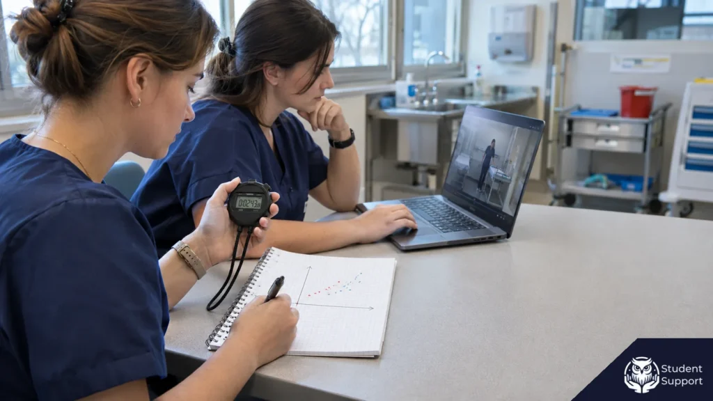
Two methods can rank results in much the same order and still give different values for the same person. In a simulation lab, a stopwatch and a video recording may both identify the same attempts as taking longer. If one reading is 47 seconds and the other 51 seconds, you need the difference in seconds to assess agreement. The Bland-Altman method describes the mean difference and estimates how far the differences extend on either side of it. The plot can also show whether discrepancies change between shorter and longer attempts.
For a thesis in “Nursing” at a university in Poland, you can use this method to ask how closely two ways of measuring the same quantity agree. This guide uses a worked exercise with ten fictional pairs of times. Each pair corresponds to one person completing a hand hygiene task once in a simulation lab. We will calculate the mean difference and limits of agreement, show how to plot the points and compare the limits with a tolerance specified before the exercise. The data and tolerance are part of the demonstration. Start by checking that both readings on each row of your spreadsheet refer to the same attempt and use the same unit.
Decide what degree of agreement you need
Write a question about the same measurement
In the exercise, one observer stands at the station and uses a stopwatch, while another later reads the time from a video of the same attempt. The question is how much the two values obtained in this way differ. In the chapter, you could ask, “How closely do live stopwatch times agree with times obtained from recordings of the same exercise in a simulation lab?” The question identifies the unit of observation, the quantity being measured and the purpose of the comparison. The reader can see that both results refer to the very same performance.
If you ask about change after training, you need measurements from two different time points. The same person may get a different result simply because they performed the task differently. Here, each person performs the task once and both values describe the same event. The study design therefore compares two recording procedures. Keeping that distinction clear also helps you name your spreadsheet columns. Use “stopwatch time” and “video time”, with a separate column for the attempt ID.
If two observers record whether a behaviour occurred as 0 or 1, you need a way to compare categorical ratings. The guide Agreement between observers in an education thesis – how to calculate Cohen’s kappa shows how to pair the ratings and assess agreement. In the Bland-Altman exercise, both observers record times in seconds. The size of the difference also matters. A difference of 1 second can affect a decision differently from a difference of 4 seconds.
Identify how you might use the result
Limits of agreement use the same unit as the measurements, so you can compare them with what the project needs. Imagine that the instructor wants to log times as the attempts take place. Later video review could provide a way to check the log if the differences were small enough for this particular task. Before comparing the results, the team specifies a range from -3 to +3 seconds. The threshold serves a teaching purpose here. It lets you work through a case in which one estimated limit falls inside the range and the other extends beyond it.
In an actual project, the reason for choosing a tolerance depends on how you plan to use the result. In the chapter, explain what accuracy that use requires, who set the threshold and what it was based on. The requirement could concern the smallest discrepancy that changes how a result is interpreted, or the accuracy needed to compare it with data from another part of the project. If you cannot justify a specific threshold, you can still describe the centre and spread of the differences. A conclusion about whether two methods can be used interchangeably requires a separate criterion.
Setting the tolerance before looking at the results makes a practical difference. If you see an upper limit of +4.58 seconds first, it is easy to choose +5 seconds and get an apparently favourable answer. State when you made the decision. If you only set the threshold after the analysis, describe the comparison as exploratory and explain your choice. A future comparison can assess a criterion set in advance.
Prepare two procedures for timing the same attempt
Agree on the start and end points
In the fictional exercise, each student completes one attempt at a simulation station. The observers use the first contact between the hands during the task as the start and the last separation of the hands after the task as the end. Flag attempts in the notes if either event is unclear. This illustrative definition is for timing the task in this demonstration. Before collecting the actual study data, try the definition on a separate set of material and decide, for example, how to handle a brief separation of the hands before the task is complete.
In procedure A, an observer starts and stops the stopwatch as the attempt takes place. In procedure B, an observer finds the start and end of the same event on the recording and subtracts the start timestamp from the end timestamp. The person reviewing the recording receives the attempt ID and the instructions used by both observers. They do not see the stopwatch reading until they have recorded their own. Knowing that the stopwatch showed 35 seconds could otherwise influence their choice of video frame when the end of the task is ambiguous.
In practice, agreement depends on the whole procedure. The stopwatch result may be affected by the observer's reaction time. The video reading may depend on the visibility of the hands, the rule for selecting a frame and the precision of the timestamps. In your conclusion about the discrepancies, name both procedures and the conditions in which you used them. Establishing measurement error for a particular device would require a different study design, usually with an independently established reference value. This exercise compares what two procedures recorded for the same event.
Keep one complete pair per person
Prepare a spreadsheet with the participant and attempt IDs, time A, time B and an indication of any missing reading. Record the unit for each result and when rounding takes place. In the exercise, all times were recorded in whole seconds and both readings were available for each person. If your timer reports minutes and seconds, convert the result to seconds before subtracting. A time of 1 min 12 s is 72 s. A value of 1.12 min is 67.2 s. The way the time is written can change the result even when every measurement was taken correctly.
Match the measurements by ID before analysing them. Sorting each time column separately preserves the individual column means but creates arbitrary new pairs. It can also change the standard deviation of the differences and the appearance of the plot. If you need to sort the spreadsheet, sort whole rows. When moving results between files, keep both values linked to the same attempt and retain the version of the instructions. Save a separate copy of the original record.
If the recording cannot be read, leave value B missing. You cannot calculate B minus A for that attempt. Record the number of attempts started, the number of complete pairs and the reasons for missing values. If the camera misses the end more often when the hands are in a particular position or when an attempt takes longer, those cases will be underrepresented among the complete pairs. Your conclusion then covers the conditions in which you were able to obtain both readings. A missing value has a different meaning from an observed time of zero.
State what a single-pair design can tell you
One pair per person lets you describe differences between the procedures in the dataset. Repeatability within each procedure requires a separate assessment. If you start the stopwatch once, that reading alone cannot show how closely it would match another reading under comparable conditions. A study of repeatability needs replicates and must distinguish change in the underlying quantity from variability within the procedure. This exercise has a narrower aim. It compares A and B for ten individual attempts.
If your thesis includes several pairs from the same person, keep both IDs and the order of the repeats. Two attempts by one person may be more similar than attempts by different people. With repeated measurements, choose an analysis that accounts for this dependence and answers your question about either a single reading or an average of readings. Bland and Altman describe separate approaches for repeated measurements. This exercise uses the single-pair formula with one observation per person.
Calculate the differences and limits of agreement for ten pairs
Read the values and state the direction of subtraction
For each attempt, subtract stopwatch time A from video time B. A positive value tells you how much longer the time from the video was. A negative value means the stopwatch gave the longer reading. Also calculate the mean of the two times for each attempt. The mean and difference become the coordinates of one point on the plot. The complete exercise dataset is below. Each item refers to a different person. All times, pair means and differences are in seconds.
- Attempt 01. A 24 s and B 26 s. The pair mean is 25 s and B minus A is +2 s.
- Attempt 02. A 28 s and B 28 s. The pair mean is 28 s and the difference is 0 s.
- Attempt 03. A 31 s and B 34 s. The pair mean is 32.5 s and the difference is +3 s.
- Attempt 04. A 35 s and B 34 s. The pair mean is 34.5 s and the difference is -1 s.
- Attempt 05. A 39 s and B 40 s. The pair mean is 39.5 s and the difference is +1 s.
- Attempt 06. A 43 s and B 41 s. The pair mean is 42 s and the difference is -2 s.
- Attempt 07. A 47 s and B 51 s. The pair mean is 49 s and the difference is +4 s.
- Attempt 08. A 50 s and B 51 s. The pair mean is 50.5 s and the difference is +1 s.
- Attempt 09. A 54 s and B 54 s. The pair mean is 54 s and the difference is 0 s.
- Attempt 10. A 58 s and B 60 s. The pair mean is 59 s and the difference is +2 s.
Work through two examples using the raw values. For attempt 03, the video time was 34 s, so 34 − 31 gives +3 s. The pair mean is (31 + 34) / 2 = 32.5 s. In attempt 06, the stopwatch showed 43 s and the video time was 41 s. The difference is 41 − 43, or -2 s, and the mean is (43 + 41) / 2 = 42 s. Write the plus sign for positive values in your working notes. This helps when you interpret the lower limit later.
The video gives the same reading of 34 s for attempts 03 and 04. The differences vary because the stopwatch readings are different. Similarly, the B reading of 51 s occurs in two separate attempts, 07 and 08. If you send two columns sorted independently, comparing the column means alone will miss the pairing error. Use rows in which both readings come from the same attempt.
Calculate the mean of the signed differences
Add all the differences with their signs. For the ten rows, the sum is 2 + 0 + 3 − 1 + 1 − 2 + 4 + 1 + 0 + 2 = 10 s. Divide by 10 to get a mean difference of +1.00 s. In this dataset, the video time is therefore one second longer on average than the stopwatch time. This is an estimate of the average shift between the two procedures. You may see it described as bias. Here it depends on the direction of subtraction and refers to this sample.
Taking the absolute values would give a different measure. If you drop the signs, the discrepancies add up to 16 s, so their mean distance from zero is 1.60 s. You can calculate this number as an additional description of the typical size of the discrepancies. The signed mean tells you which procedure gave a longer time on average. For the standard limits of agreement, use +1.00 s and the standard deviation of those same signed differences.
Calculate the standard deviation of the differences
Subtract the mean of +1 s from each difference. In attempt order, you get 1, -1, 2, -2, 0, -3, 3, 0, -1 and 1 s. The +4 s difference for attempt 07 lies 3 s above the mean. The -2 s difference for attempt 06 lies 3 s below it. After squaring the deviations, both rows contribute 9 s². Sum all the squared deviations. In this example, the total is 30 s².
For the sample calculation, divide 30 s² by the number of pairs minus one, which is 9. The sample variance is approximately 3.3333 s². Taking the square root gives a standard deviation of about 1.82574 s. In a spreadsheet, apply the sample standard deviation function to the differences column. If the result is about 1.73205 s, you probably used the version that divides by 10. Check the function and the cell range. The mean difference depends on the signs. In this step, spread depends on distance from the mean, so both positive and negative deviations contribute.
The standard deviations of A times, B times and pair means describe how long different people took to perform the task. For the limits of agreement, you need the spread of the differences. In this example, the readings for different people range from 24 to 60 seconds across the two procedures. That range alone tells you little about how much the procedures differ within a single attempt. The calculation from the differences column answers that question.
Substitute the values and interpret the sign of each limit
For the standard method, subtract 1.96 standard deviations from the mean difference and add the same amount to obtain the approximate 95% limits of agreement. Multiply the standard deviation by 1.96 to get approximately 3.57845 s. Substituting the mean of +1 s gives the following values.
- Lower limit of agreement. 1.00 − 3.57845 ≈ -2.58 s.
- Mean difference. +1.00 s for the video time relative to the stopwatch.
- Upper limit of agreement. 1.00 + 3.57845 ≈ +4.58 s.
The limits are symmetric around +1.00 s. Zero is below the centre line, so the limits are asymmetric around zero. The lower limit extends into the range where the video time is shorter. The upper limit shows that the estimated range extends further into the range where the video time is longer than the stopwatch reading. Report the limits in this order, state the direction of subtraction and give the unit.
If you calculate A minus B, every signed difference changes sign. The mean becomes -1.00 s and the limits, ordered from lower to upper, run from -4.58 to +2.58 s. The spread stays the same. This version is valid if the plot labels, values and interpretation all use the same convention. When reviewing the finished chapter, find a sentence that links the sign to the longer reading. This lets you check whether the plot and the text agree.
Plot the results and read an individual attempt
Put the pair mean on the horizontal axis
Create a scatter plot from the two columns you calculated. The horizontal axis shows the mean of the two readings for an attempt. The vertical axis shows B minus A. The point for attempt 03 has coordinates 32.5 s and +3 s. Attempt 06 sits at 42 s on the horizontal axis and -2 s on the vertical axis. Attempt 07 gives the point at 49 s and +4 s. The matching readings of 28/28 s and 54/54 s both sit at zero on the vertical axis, each at a different mean time. They are distinct points for two separate attempts.
Label the horizontal axis “Mean time from the two methods (s)” and the vertical axis “Video time minus stopwatch time (s)”. The labels should make the plot readable on its own. Equal readings give a vertical value of zero. Points above zero represent attempts with longer video times. Points below zero represent attempts with longer stopwatch times. Both axes use seconds, with a different quantity on each axis.
You can use a horizontal line for the mean of +1.00 s and dashed lines for the limits at -2.58 and +4.58 s. A line at zero makes the sign of each difference easier to read. Use a label and line style that distinguish it from the mean. If you add the tolerance from -3 to +3 s, give it a different style and explain where it came from. If two lines are close together, you can give some of the values in the figure caption. Make sure the reader can tell which line comes from the data and which represents the project's threshold.
Look for a pattern in the differences
Start by checking where the points are centred. In this example, the mean is +1.00 s, although several readings fall at or below zero. Then look across the points from left to right. The short attempt 03 has a positive difference of +3 s, attempt 06 in the middle of the range gives -2 s, and attempt 07, with a mean of 49 s, gives +4 s. The longer attempts also include differences of 0 s and +2 s. These ten pairs show no clearly consistent increase in the difference as time increases. This observation applies to the dataset shown.
Also check whether the vertical spread widens at large values. If short attempts have small differences while long attempts have both large positive and large negative differences, one set of limits may describe the overall range poorly. If the points shift upwards without much change in spread, the average difference is changing. These patterns raise different questions about the procedure and analysis. With ten points, a single point can also create the appearance of a trend, so describe the visible pattern cautiously.
In a thesis, check whether the model fits beyond what you can see on the plot. The standard formula assumes that the differences are approximately normally distributed and that their mean and spread do not change substantially with measurement size. The method also assumes that the differences from separate pairs are independent. The distributions of times A and B are separate considerations. Inspect the distribution of the differences and check any unusually large or small points. In a small sample, a formal normality test has limited power to detect departures, and the absence of an obvious pattern tells you little about how stable the limits are. Treat the calculations and plot in this exercise as an illustration of the method.
If you see a pronounced trend or a changing spread, revisit the measurement procedure and your hypothesis. It might be harder to identify the start or end of longer attempts. Sometimes the pattern reflects how the procedures operate. Bland and Altman's 1999 paper discusses ways to handle differences that depend on measurement size, including transformation and modelling. Your choice changes how you report the result and needs a rationale. For a simple illustration, explain when a common set of limits would be unsuitable and check whether your data suggest that problem.
Compare the result with the project's tolerance
Read both limits
In the exercise, we set an acceptable range of -3 to +3 s. The lower limit of agreement of -2.58 s lies within the range by about 0.42 s. The upper limit of +4.58 s exceeds the threshold by about 1.58 s. The mean of +1 s lies within the tolerance. A conclusion about agreement for individual attempts requires checking both limits. The calculation therefore addresses a practical question for the team considering the two methods for the same task. The point estimates of the limits do not both fall within the demonstration's acceptable range.
You can also count how many observed differences fall outside the tolerance. If the endpoints are included, attempt 03, at +3 s, is at the upper boundary and attempt 07, at +4 s, exceeds it. Nine out of ten pairs are within tolerance. This proportion describes the data in the exercise. In an actual study, the proportion meeting the criterion and the estimated limits of agreement can be reported separately. The proportion tells you how many recorded differences met the criterion. The limits use the mean and standard deviation of the differences to describe the spread expected under the model.
Distinguish expected spread from uncertainty in the limits
Under the relevant assumptions, the interval between the limits is intended to cover about 95% of the distribution of differences for measurements made under similar conditions. That is the quantity you are estimating. A finite sample gives approximate values for the limits. In this example, all observed differences, from -2 to +4 s, lie within the estimated interval of -2.58 to +4.58 s. With ten pairs, each point represents 10% of the observations and the observed proportion inside the estimated interval is free to vary.
You can describe estimation uncertainty with separate confidence intervals for the lower and upper limits. Their width depends on factors such as the sample size, the spread and the method used to calculate them. If a study is designed to assess whether methods can be used interchangeably, consider whether the estimates are precise enough to support that decision. Even if both point estimates lie within the tolerance, their confidence intervals may extend further. This exercise does not calculate those intervals. The upper point estimate already exceeds the threshold, and the ten fictional pairs illustrate how to read the result.
A confidence interval for the mean difference describes uncertainty in the average shift. You can estimate that shift precisely and still see a wide spread of differences within individual pairs. When you write “95%”, say what it refers to. For the limits of agreement, it refers to the approximate coverage of the distribution of differences under the model. For a confidence interval, the confidence level refers to the procedure for estimating an unknown parameter such as the upper limit or the mean difference.
Check what a high correlation tells you
For the fictional A and B times, Pearson's correlation is approximately 0.988. Attempts that take longer according to the stopwatch usually take longer according to the video too. This is consistent with a high correlation. At the same time, the procedures differ by 4 s for attempt 07 and the upper limit calculated earlier is +4.58 s. These results can occur together. The correlation describes how the two readings vary together, while the limits describe how far apart they can be in seconds.
Consider a simple thought experiment. If every video time were exactly 5 seconds longer than the stopwatch time, the correlation would be 1 as long as the times varied across attempts. Each pair would differ by 5 seconds. If the application tolerates a difference of only 3 seconds, the identical ranking of attempts would still fail the criterion. Bland and Altman showed in their 1986 article that the range of the measured values can strongly influence the correlation. In this exercise, the times span several dozen seconds, which favours a high correlation even when some discrepancies matter to the project.
A test of the mean difference also answers a different question. A small mean can arise when positive and negative differences cancel each other out. Individual discrepancies may still exceed the project's threshold. When preparing the results for your instructor or supervisor, start with the question about an individual reading. If the question is how far the two readings could differ for one attempt, report the limits of agreement, the unit and the direction of subtraction.
Report the method, result and limitations in your thesis
Describe the conditions needed to reproduce the method
In your methods paragraph, describe the quantity measured by both procedures, the unit of observation and the number of readings per person. State what marked the start and end, and who recorded those events and when for each method. Explain how you read the timestamps and state the unit and precision. A reader should be able to tell whether the stopwatch and the recording describe exactly the same attempt. If recording differed from the research plan, report what actually happened and explain the implications for the comparison.
The methods paragraph for this demonstration could read as follows. “The calculations used ten fictional pairs of times, each representing a single attempt. Time A was recorded live with a stopwatch, and time B was determined from the start and end timestamps of the same attempt. Both procedures used the same definitions of start and end. The observer who reviewed the recording was unaware of measurement A. Agreement was described using the mean difference B minus A, the standard deviation of differences, and the approximate 95% limits of agreement calculated as the mean difference ± 1.96 standard deviations of the differences. A teaching tolerance from -3 to +3 s was specified before the comparison.”
For a thesis with real data, include the number of attempts with incomplete readings and explain how you handled them. If observers changed between sessions, explain their role and say which attempts each assessed. This detail can help explain where some variability comes from. Keep the methods distinct from the discussion. The methods describe what you did so that a reader could reproduce it. The discussion can assess to what extent your design reflects the intended use.
Give the values, direction and unit in the results
An example for the results section is as follows. “Across ten complete pairs, the mean difference between video time and stopwatch time was +1.00 s (standard deviation of the differences 1.83 s). The estimated 95% limits of agreement ranged from -2.58 to +4.58 s. The plot showed no clear pattern in the differences as the average time increased, an observation based on ten fictional pairs. The upper limit exceeded the prespecified threshold of +3 s.” If the proportion within tolerance answers a separate question, add that 9 out of 10 pairs fell within the range when its endpoints were included.
If you are describing results from a published paper, check how the authors defined the limits and the direction of the difference. One study may subtract the existing method from the new method and another may use the reverse order. Check the direction of subtraction, units and measurement conditions before comparing the ranges. The fact that two studies used a Bland-Altman plot does not establish that their values are directly comparable.
Explain the scope of the conclusion in the discussion
The exercise asks about two ways of timing the same task. Under the stated tolerance, the upper estimated limit is too high for these results to support using the two procedures interchangeably in this demonstration. Establishing the true duration would require a reference measurement beyond the two readings. Assessing the repeatability of either procedure would require its own design. These distinctions tell you what an expanded study would need to establish.
For educational use, the range of timings and the recording conditions matter. Results could change with a different camera position, a different group of observers or a different way of identifying the end of the task. Replace “the video method overestimates the time” with a specific statement. “In this demonstration, the video reading was 1.00 s longer on average than the stopwatch reading.” This wording makes the origin of the number clear. If discussing what might have caused the difference, identify possible mechanisms and say what further observations would allow you to investigate them.
Check each step from the research question to the plot labels
- Read your research question out loud. It should identify two methods measuring the same quantity in the same attempt.
- Open one row with a positive difference and one with a negative difference. Check the ID, units and direction of subtraction.
- Recalculate the standard deviation using the differences column. Try reproducing one limit from unrounded values.
- Compare the vertical axis label with the results in the text. If a positive value means a longer video time, use the same interpretation in the discussion.
- Keep the estimated limits of agreement separate from the project's threshold. Make sure the methods describe how and when you set the threshold.
- State how many attempts had complete readings, what range of times the data covered and whether the observations came from different people. Set the scope of the conclusion accordingly.
Questions about the plot, sample size and statistical support
Is a description needed for every chart?
The result should be discussed in the text, but the commentary does not need to repeat every value. Highlight the key finding and its connection to the research question. Avoid including a series of charts without explaining why they are shown.
How can I connect a limitation to its effect on the conclusions?
Identify a specific feature of the procedure, the finding or claim it affects, and the consequence. Then explain what you actually did to address it and what remains uncertain. A generic list mentioning sample size and time pressure is not enough.
How many people are needed for statistical analysis in a master's thesis?
There is no single number suitable for every thesis. The planned test, the number and size of groups, the expected effect size, and the required power and precision of the analysis are important. A small sample limits inference. It is best to discuss the sample size before starting data collection.
When should I use Pearson's correlation and when Spearman's?
Example: are higher stress levels associated with lower satisfaction? Pearson's correlation describes a linear relationship between quantitative variables. Spearman's correlation is based on ranks and assesses monotonic relationships, including those involving ordinal data. Before selecting the method, I will consider the measurement scale. I will check the scatter plot and the possible influence of outliers. Correlation alone does not establish causation.
How much does statistical analysis for a degree thesis cost?
I will prepare a quote after reviewing the database and research questions. The cost depends on data cleaning, the number and complexity of analyses, the scope of tables and description, and the deadline. I do not price the service based solely on the number of pages in the thesis.
What will I receive after the statistical analysis is completed?
I agree the scope before starting. It may include a prepared dataset, descriptive statistics, test results, tables, charts, a description of the methods and interpretation in relation to the research questions. I agree the format of editable files and any materials from the software when I prepare the quote.
Sources
- Bland, J. M., Altman, D. G. (1986). Statistical methods for assessing agreement between two methods of clinical measurement. The Lancet, 327(8476), 307-310. DOI
10.1016/S0140-6736(86)90837-8. Full texthttps://jhanley.biostat.mcgill.ca/c678/b%26a.pdf. - Bland, J. M., Altman, D. G. (1999). Measuring agreement in method comparison studies. Statistical Methods in Medical Research, 8(2), 135-160. DOI
10.1177/096228029900800204. Full texthttps://bendixcarstensen.com/MethComp/Papers/Bland.1999.pdf. - Wilczyński, M. Konspekt ze statystyki. Wrocław University of Science and Technology, chapter 13, “Metoda Blanda-Altmana”.
https://alfa.im.pwr.edu.pl/~wilczyn/badanie%20wzroku/konspekt%20ze%20statystyki%202019.pdf. - Chen, J., Yang, L., Mak, Y.-W., O’Donoghue, M., Shi, C., Tsang, H., Lu, S., Zou, J., Qin, J., Xie, Y. J., Lai, T., Li, C., Cao, J., Pittet, D. (2024). Hand Hygiene Education Components Among First-Year Nursing Students: A Cluster Randomized Clinical Trial. JAMA Network Open, 7(6), e2413835. DOI
10.1001/jamanetworkopen.2024.13835. Full texthttps://pmc.ncbi.nlm.nih.gov/articles/PMC11177166/. In the study of 270 first-year nursing students in Hong Kong, experts assessed the duration of individual steps from video recordings. The stopwatch comparison and the numbers in this guide were created for the exercise.
Do you need to describe agreement between two methods in your thesis?
Send your research question, measurement instructions, pairs of readings with identifying information removed, and a draft plot if you have one. We can check your differences and limits of agreement and help you draw a conclusion that reflects the scope of your study.
Discuss your analysis with StudentSupport